How to Handle Census Tract Data: A Reporter’s Guide (2026)

If you are wondering how to handle census tract data, the answer is narrower than it sounds: it comes down to one join. Census publishes tract boundaries as a geometry file and tract attributes as a separate table, and the two only meet when you match them on an 11-digit GEOID. Get that key right and the rest — cleaning, normalizing, mapping, documenting — takes about an hour. Get it wrong and you publish a map of nulls, or worse, a map that looks fine and is quietly wrong.

This guide is written for reporters and newsroom developers working under deadline. It assumes you have a story question, a pile of addresses or point records, and a need for neighborhood-level demographics. It does not assume you write Python. Where a script helps, you will get a short one, and where clicking works, you get that too.

One more thing worth saying up front: most tract-level numbers are estimates, not counts. A tract can hold 4,000 people and still be too small for a reliable survey estimate, which is why the American Community Survey ships a margin of error alongside every figure. Learning to handle census tract data well means handling that uncertainty honestly.

What You Need

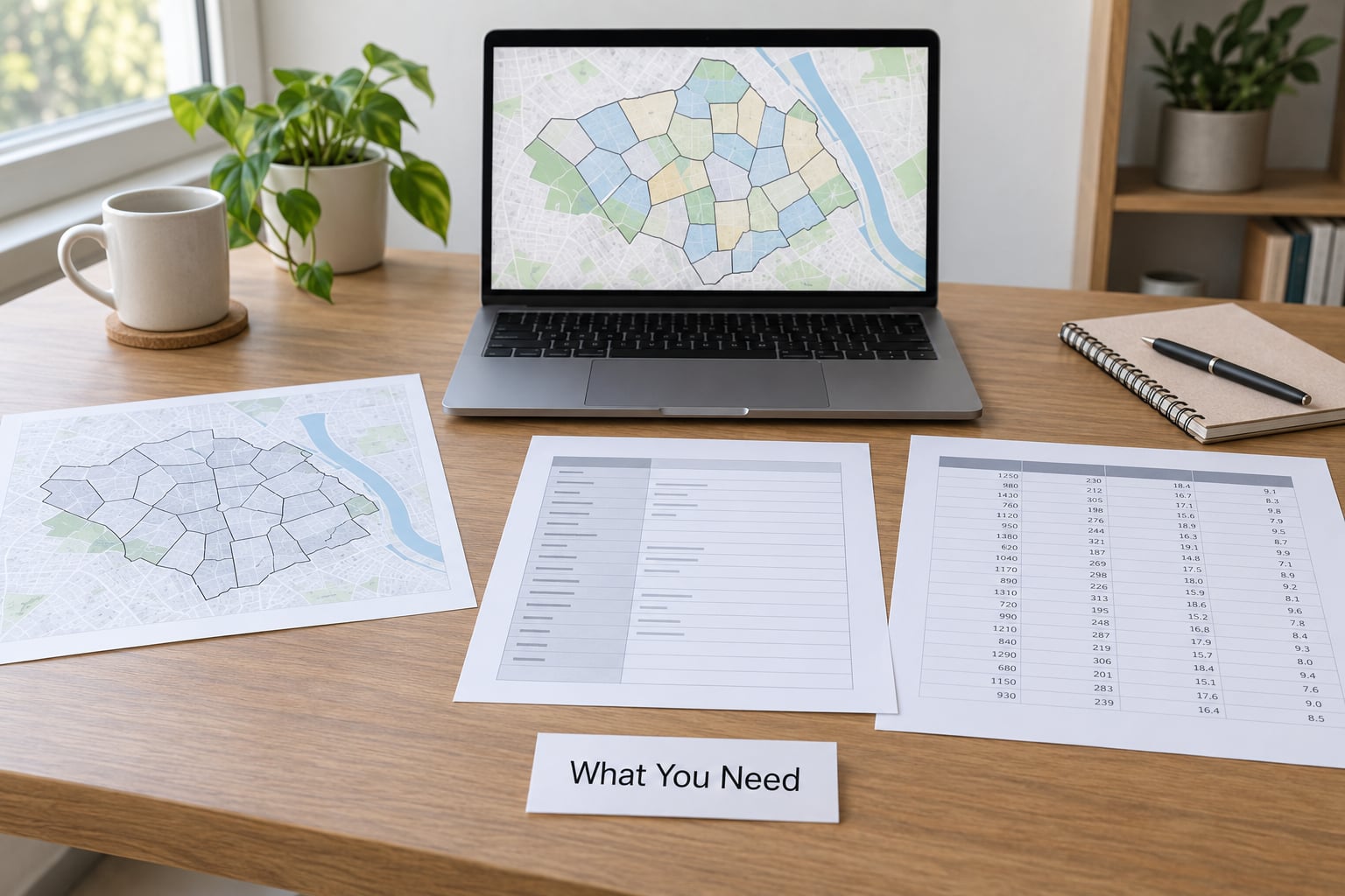
Five things, and you can assemble them in any order. Missing any one of them is what produces the frustrating hours later in the process.

Boundary files. Census geometry comes from TIGER/Line, which is the Census Bureau’s cartographic files of state, county, tract, block group and block boundaries. Grab the tract layer for your states, not the county layer — the tracts are nested inside the counties and come with their own attributes such as land area and water area.

An attribute table. This is the actual census tract data: population, households, income, race, tenure, whatever your story needs. It can come from data.census.gov, the Census API, or a bulk download such as the decennial Detailed DHC-B tables or an ACS subject table. Pick one and write down its identifier.

Lookup and crosswalk files. These are the files that translate between geographies. The block relationship files translate blocks to block groups and tracts. The ZCTA relationship file translates ZIP-based areas to tracts. The NHGIS crosswalk tables translate an old vintage of tracts to a new one. Most “I cannot find my neighborhood” problems end at one of these three.

A reproducible environment. That means a project folder, a script or a documented set of clicks, and files that are re-downloadable by someone else. If your only copy of the data is a file a colleague emailed you, you cannot publish responsibly.

A mapping tool and something to read the docs. QGIS is free and does everything in this workflow. So do ArcGIS Pro, Tableau and even a well-built spreadsheet for small jobs. Pair it with the table shell layout, which is the single most useful page for decoding column names like B01003_001E.

Before you start, write down the vintage you are working with. Census publishes a new decennial geography roughly every ten years, and the tract boundaries you download today are not the tracts that existed ten years ago. The vintage is the first thing a fact-checker will ask about.

Worth knowing which route costs what, because the choice changes your deadline. A one-off lookup for a single neighborhood is a few minutes on data.census.gov. A full story map for one metro is usually faster through the API, because you write the request once and reuse it. A multi-county or nationwide project, or anything involving a past decade, is an NHGIS job and a longer afternoon. The manual download path does not become wrong at scale, it just stops being free.

Step-by-Step

1. Define the geography before you touch census tract data

A census tract is a small, relatively permanent subdivision of a county or county equivalent, holding roughly 1,000 to 8,000 people with an optimum size near 4,000. Tracts are designed to follow visible features like roads, rivers and rail lines, and they are redrawn each decade to keep populations comparable. Crucially, a tract never crosses a county line — every tract belongs to exactly one county, which is why the county FIPS code is part of its identifier.

That stability is the reason tracts became the default unit for neighborhood analysis. The downside is size: a tract in a dense city can hold 1,000 people, a rural tract can hold 8,000, and comparing raw counts between the two is meaningless. Block groups are the finer step inside a tract, typically 600 to 3,000 people. Blocks are the smallest published unit, and they are not stable enough to compare across decades. Deciding which unit you are actually reporting is the first real decision in how to handle census tract data.

Choosing the unit is a real editorial decision, and it is usually the root cause of a bad result. Practitioners on GIS and data forums keep landing on the same point: the spatial unit, not the statistic, is what quietly ruins most neighborhood analysis.

Unit	Typical population	Stable across decades	Best for	Key limitation
Census tract	1,000 to 8,000	Yes, roughly	Neighborhood comparison, environmental justice, health outcomes	Redrawn each decade, so decade-over-decade comparison needs a crosswalk
Block group	600 to 3,000	Partly	Sub-neighborhood detail where a tract is too coarse	More survey noise per estimate, and many cells suppressed
Census block	Varies, often 10 to 100	No	Point-to-area allocation, precinct matching	Never publish block-level figures; disclosure avoidance blurs them
ZCTA	Varies widely	Roughly	Connecting to ZIP-based administrative or business data	Not a census geography in the statistical sense; huge size variation
H3 hexagon	Set by resolution, not by people	Yes	Uniform national or global coverage, custom density	Ignores real boundaries; you must allocate tract data into hexagons yourself
County	Thousands to millions	Yes	Denominators, rural context, top-line totals	Far too coarse for a neighborhood story

Then decide what kind of number you are reporting. A count says how many people. A rate normalizes by a denominator, such as rate per 1,000 residents. A percentage normalizes within the tract, which can be misleading when the denominator is tiny. If your story is about risk, incidence or disparity, you almost always want a rate built on a stable county-level or state-level denominator, with the tract supplying the numerator.

Write the geography on one line in your notes — unit, vintage, table ID — before you download anything. You will repeat that line in the caption, and repeating it is free.

2. Download the correct Census data and boundary files

Three datasets cover almost all tract work, and they are not interchangeable.

The decennial Census is a complete count taken every ten years. It is the most accurate population count available and the right source for redistricting and for “how many people live here” questions. The 2020 Detailed DHC-B tables publish at tract level and include a wide set of race, ethnicity, household and housing variables.

The American Community Survey 1-year estimates cover every tract in the country, with a sample large enough for metro areas and larger cities but too thin in rural areas. The 5-year estimates pool five years of survey data, which produces wider geography coverage and smaller margins of error at the cost of a blunter time picture. As a working rule, use 1-year where your geography is metropolitan, 5-year where it is rural or small-town, and never mix the two vintages in one map.

Where you get them: data.census.gov is the official front door and it will hand you a table with a shareable link. The Census API returns JSON or CSV for the same tables and is the better choice once you know your table IDs. TIGER/Line is the source for geometry, in shapefile or GeoJSON form. For anything pre-2020, NHGIS is the only sane route to historical tract data on consistent boundaries.

In R or Python, tidycensus does the whole download-and-join in two calls:

library(tidycensus)
tracts <- get_acs(variables = "B01003_001E", year = 2023,
                 geography = "tract", state = "NY")
tracts <- tracts %>% filter(GEOID != "")

Check before you proceed: does the table’s geography match the shape file’s vintage, and does every tract in the table have a matching polygon? A mismatch here produces a partial join that looks fine until you count the nulls.

3. Clean identifiers and field names, including the 11-digit GEOID

This is the step that eats people’s afternoons, and the fix is mechanical. Most of how to handle census tract data is bookkeeping, and this is where it usually breaks. The 11-digit tract GEOID is three codes concatenated:

1. State FIPS code, 2 digits — for example 36 for New York.
2. County FIPS code, 3 digits, zero-padded within the state — for example 061 for New York County (Manhattan).
3. Tract number, 6 digits, zero-padded — for example 023100.

Stitched together, that is 36061023100: 2 digits plus 3 plus 6. It reads unambiguously as state 36, county 061, tract 023100. Every ACS and decennial tract table carries this key, and every TIGER/Line tract layer carries the same value in its GEOID field. When you download, write it down both ways so you can decode a stray identifier later.

Four cleaning rules, in order:

Keep identifiers as text. The moment 36061023100 becomes a number, the leading zeros inside 023100 vanish and the join fails silently — no error, just a column of empty cells. Force the column to string on import.

Load the type definitions. Census data downloads include a small file describing each column as text, integer or float. Loading it stops a spreadsheet from guessing wrong and stops 11-digit identifiers from being mangled.

Watch the 10-character limit. The classic failure comes from converting GeoJSON or API output into a shapefile, which truncates field names to 10 characters. A key called census_tract or GEOID_2020 becomes something else entirely, and the join quietly finds nothing. Use GeoPackage or File Geodatabase as the working format if you can, or rename the field to something short and identical on both sides before you convert.

Inspect the empties before you analyze. Suppressed cells are not zeros, and a missing value is not a zero. Filter out geography with zero land area, since water-only tracts will pollute any average. Count how many records came back empty and decide deliberately what to do with them.

You can tell which summary level you actually have from the summary level code, and the number you want for tracts is 140. Block groups are 150, blocks are 101, counties are 050. If your file reports a different summary level than you expected, stop and check which download you actually took.

4. Join demographic data to tract boundaries

With matching keys, the join is one operation. What matters is verifying it rather than assuming it. After joining, count rows on both sides. If the joined table has fewer rows than the boundary file, some tracts had no attributes; if it has more, your key is not unique and you have a fan-out. Inspect the unmatched records and decide whether they are genuinely empty or a symptom of a key mismatch.

Use a table join on the 11-digit GEOID when your attributes are already tract-level. Reach for a spatial join only when your data starts as points or as a different geography — a list of addresses, for example — and in that case treat the spatial join as a separate step with its own accuracy problem: the tract you get is the tract containing the point, which may be a different tract than the tract containing the household behind the address.

If your attributes and your shapes come from different vintages, stop. A 2010-vintage tract table joined to a 2020-vintage shape will either fail to match or, worse, match the wrong polygon. Pick one vintage for both, or use a crosswalk and document it.

5. Calculate rates, percentages, and uncertainty

Normalize before you map. A tract map colored by raw count is a population density map wearing a costume, and readers will read it as a rate. For a rate, keep the numerator at tract level and pull the denominator from a larger geography — the county, the metro area, the state — so a single unusually small tract does not produce a wild number.

Guard the denominator. Divide by zero, and by denominators small enough that the ratio is noise. A sensible publication rule: do not report a percentage for a group whose estimated count is below a few dozen, and say so in the methodology rather than quietly dropping those tracts from the map.

Handle the margin of error explicitly. Every ACS estimate arrives with a companion margin-of-error column, and a difference between two tracts is only meaningful when the two estimates do not overlap within their margins. A workable threshold for publication: if the margin of error exceeds roughly 10 to 15 percent of the estimate, either present the range or move up a geography. You will see this constantly in rural tracts, where the sample is thin. It is also why suppressed cells exist: the Census Bureau withholds values where disclosure avoidance rules would let someone be identified.

6. Map the results and test the display

Choose the classification deliberately. Quantile puts the same number of tracts in each color band, which makes the map look evenly textured but hides the extremes. Natural breaks groups similar values together and usually shows real clustering. Equal interval is the most common source of a misleading map, because one outlier flattens everything else into a single shade. If your story is about a threshold, map the threshold as two categories rather than as a gradient.

Label the map with something a reader can orient by — a county outline, a city label, a scale bar — and keep the color scheme consistent across every map in the series. Then look at the map again and ask whether the visual pattern is a pattern in the data or an artifact of the classification. If you swap the classification and the story changes, you do not have a story.

Finally, zoom in on your outliers. The one tract that dominates the color scale is usually a water-only tract, a university campus with a strange housing count, or a prison. Figure out which, then decide whether it belongs in the frame.

7. Document, reproduce, and publish

Documentation is not paperwork; it is the thing that saves you when a reader emails with a question at 10 p.m. For every map and table, record the dataset name and vintage, the table ID, the variables used, the geography unit, the projection, the vintage of the boundary file, and the margin-of-error handling you chose.

Comparing two decennia needs one extra step. Because tract boundaries were redrawn between 2010 and 2020, a naive comparison of “tract 023100 in 2010” against “tract 023100 in 2020” is comparing different places. The fix is backcasting: use the block-level relationship files, or the NHGIS crosswalk tables, to distribute the earlier data onto the later geography. You are then reporting “this area, as defined today” rather than “this tract number”. Those are different sentences and your caption should say which one you wrote.

A short checklist for the published graphic: vintage year, dataset, table ID, unit of analysis, projection, denominator for any rate, and one sentence on margin of error. A newsroom that puts these in the caption stops the “where did this number come from” email before it starts.

Common Mistakes

Almost every failed tract project I have seen traces back to one of eight things. The first three are join failures, and they produce the same symptom for different reasons.

Symptom	Likely cause	Fix
Every value is null after a join	Key imported as a number, so leading zeros dropped	Re-import the column as text and re-check the length is 11 characters
Some tracts match, some do not	Attributes and shapes are from different vintages	Use one vintage for both, or run a crosswalk and document it
Row count explodes after joining	Duplicate keys on one side, often a tract-level file joined to a block-level file	Aggregate to one row per 11-digit GEOID before joining
Join key field keeps changing name	Field names truncated to 10 characters on conversion to shapefile	Rename the key to a short identical name, or work in GeoPackage
Map looks dramatic, story collapses	Raw counts mapped instead of rates	Normalize against a stable larger geography and re-map
Some values are blank with no warning	Suppressed cells from disclosure avoidance	Treat as missing, not zero, and say so in the methodology
One tract owns the entire color scale	Water-only tract with zero land area	Filter on zero land area and re-classify
Decade-over-decade trend is nonsense	Comparing redrawn tract boundaries directly	Backcast older data onto current boundaries with a crosswalk

Two more errors that never show up as a broken map, which is what makes them dangerous. The first is reading an ACS estimate as a headcount. It is a survey-based estimate with a margin of error, and publishing “1,240 households” when the real figure might be 1,090 to 1,390 is a factual error even though the point estimate is technically the published number.

The second is treating block-level data as individual-level data. Blocks exist for operational purposes and disclosure avoidance deliberately obscures small counts, so a block-level figure is fuzzy by design. If you need block-level detail for a boundary-crossing problem, use it as a weighting step to allocate into block groups or tracts, and publish at the level the data can actually support.

And a habit worth dropping early: treating ZIP codes as interchangeable with census geography. ZIP codes are postal delivery routes, they overlap, and their population varies enormously. Practitioners argue about this constantly on GIS forums and they are right. If your source data is ZIP-based, crosswalk it to ZCTAs and then allocate to tracts by overlap weight, and say that you did.

Frequently Asked Questions

Conclusion

Start with five things, in this order. Write down the geography and the vintage before downloading anything, so every later decision has a fixed reference. Pull the tract boundaries and the attribute table from the same vintage, and confirm the boundary layer is summary level 140. Treat the 11-digit GEOID as text and never let a spreadsheet turn it into a number. Look at your margins of error and your suppressed cells before you believe any result. Then write the caption — dataset, vintage, table ID, unit, margin-of-error handling — while the details are still in front of you.

Most of the difficulty in how to handle census tract data is bookkeeping, not statistics, and bookkeeping gets easy once it is a checklist. The story you can tell afterward is the reward.