How to Use Pandas for Data Journalism: A Practical Guide 2026

To use pandas for data journalism, you load a public data file into a DataFrame, inspect it before you touch it, clean it with recorded decisions, answer one reporting question at a time with grouped calculations, then reconcile every number against the original source before it goes anywhere near a headline. The tool itself is the easy part. The part that makes a story defensible is the discipline around it.

This guide walks through that workflow in six steps, using a city’s 311 service request export as the running example. The output shown under each code block comes from a small illustrative extract, so your totals will look different from the moment you download your own file.

What You Need

You need four things before you write a single line of code: Python, pandas, somewhere to run it, and the documentation that shipped with the dataset.

Python and pandas. Pandas is a library, so it lives inside Python. Install both from the terminal with pip install pandas jupyter, then confirm it works by running python -c "import pandas as pd; print(pd.__version__)". If that prints a version number, you are ready.

A place to run code. Jupyter notebooks are the usual choice for reporting work because each cell runs, displays its result, and stays in order. Google Colab runs the same notebooks in a browser with nothing installed locally, which is useful when you are on a deadline laptop or want to share a link with an editor. If you prefer plain files, a script and a code editor work just as well, they just show you less as you go.

A folder that keeps raw data untouched. Give every story its own folder with three subfolders: raw for the untouched download, clean for the cleaned version, and output for tables and charts. Write to clean and output only. The raw copy is the copy you check your totals against, and it is the copy that proves what you did and did not change.

The source documentation. Every serious dataset arrives with a data dictionary or a notes page explaining what each column means, how often it updates, and known gaps. Save it next to the raw file. A column called case_nbr means something different in every city, and guessing changes the meaning of your story.

Step-by-Step

1. Set Up a Reproducible Pandas Environment

A reproducible environment is just one where someone else, including you next month, can run your analysis again and get the same numbers.

Create the notebook inside your story folder, import pandas under the short alias everyone uses, and print the version at the top of the notebook so your output records which pandas produced it.

import pandas as pd
print(pd.__version__)

What to look for: a version string such as 2.2.3. That line in the notebook is your first reproducibility record, and it costs one cell.

2. Import the Data and Inspect Its Structure

Load the file with read_csv and inspect the DataFrame before changing anything, because the shape of the data dictates every step that follows.

requests = pd.read_csv("raw/311_requests.csv")
requests.head()
requests.shape
requests.info()
requests.dtypes
requests["category"].value_counts().head(10)

What to look for: shape gives you rows and columns, info shows how many values are missing in each column, dtypes tells you whether a date arrived as text, and value_counts shows the categories you will actually group by later. A file whose date column reads object instead of datetime64 has not been parsed yet, and that matters on the very first line of any time-based finding.

Not every file is a CSV. read_excel handles multi-sheet workbooks and read_json handles API responses, and both return the same DataFrame object once loaded.

3. Clean Types, Missing Values, Duplicates, and Outliers

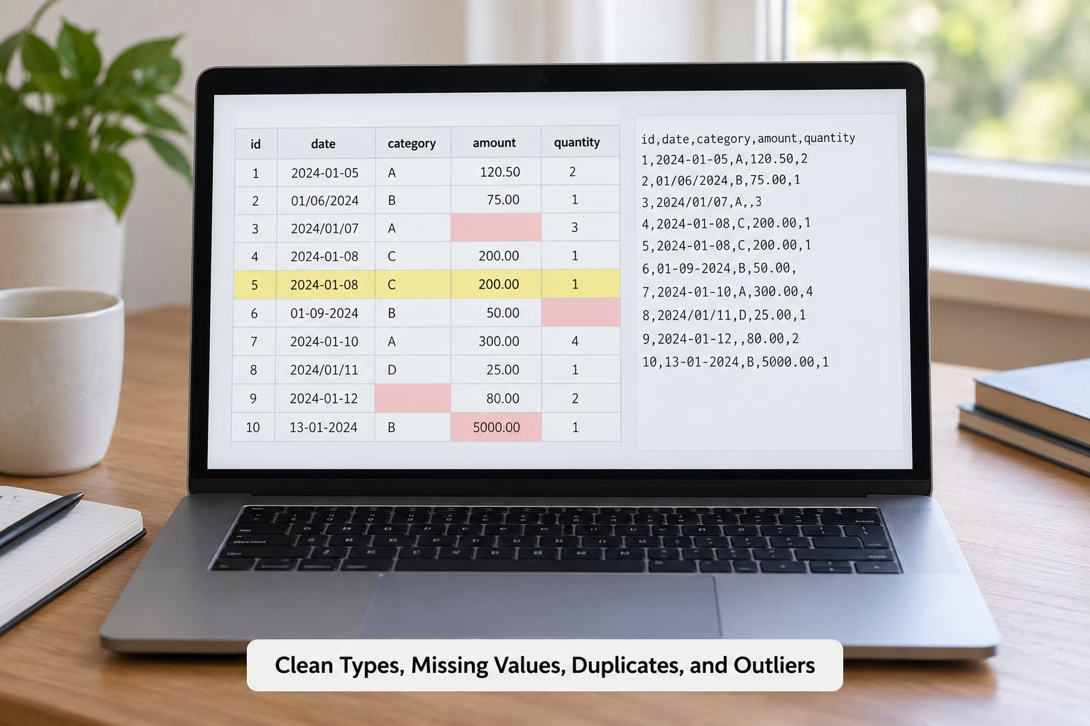
Clean the data in code, on a copy, and write down each decision you make, because cleaning that nobody can reconstruct is indistinguishable from data massaging.

Convert dates properly, force columns that should be numbers to become numbers, decide what a missing value means, and remove duplicate rows:

requests["opened"] = pd.to_datetime(requests["opened"], errors="coerce")
requests["closed_gap_days"] = pd.to_numeric(requests["closed_gap_days"], errors="coerce")
requests["zip"] = requests["zip"].astype(str).str.zfill(5)
requests = requests.drop_duplicates(subset=["request_id"])
requests.isna().sum().sort_values(ascending=False).head()

What to look for: errors="coerce" turns unparseable dates into missing values rather than crashing the notebook, and isna().sum() ranks the columns with the biggest gaps so you know where to look first. If a column used -1, 999 or N/A to mean unknown, pass those to na_values at load time so they never enter your arithmetic as real figures.

Outliers need judgement, not a reflex. A 900-day closure time is usually a data error, but a city that genuinely closed one request after three years is a story in itself, so check the extreme rows by eye before you delete anything.

4. Ask and Answer Data Questions with Grouped Analysis

Turn your reporting question into one specific pandas operation, rather than sorting and plotting everything to see what falls out.

Filter rows with a boolean mask, pull values with loc and iloc, then group and aggregate:

picked = requests[(requests["category"] == "Pothole") & (requests["borough"] == "North")]
picked.sort_values("opened").head()

by_month = (requests.dropna(subset=["opened"])
                   .set_index("opened")
                   .resample("MS")
                   .size())
requests.groupby("borough")["closed_gap_days"].agg(["count", "median"]).round(1)

What to look for: groupby(...).agg() gives you the median closure gap per borough, which is far more readable in a story than a mean dragged upward by a few very old cases. pivot_table does the same thing in two dimensions when you want categories down the side and boroughs across the top.

Raw counts mislead. A borough with more complaints is often simply the borough with more residents, so divide by population before you write that one area is worse than another:

rates = (by_category.assign(per_100k=by_category["count"] / by_category["population"] * 100_000))
rates.sort_values("per_100k", ascending=False)

5. Validate Results Before Publishing

Validate every result before publishing by reconciling it against the source, because a chart that disagrees with the agency’s own table is the fastest way to lose a correction.

Run these four checks before you write anything down:

1. Reconcile the totals. Sum your cleaned table and compare it with the row count or headline figure published alongside the raw file. If they differ, you dropped rows and need to know which and why.
2. Test the date range. Print requests["opened"].min() and .max() and confirm they match the period you intend to describe. Off-by-one month errors are easy and invisible.
3. Read representative rows. Pull ten random rows with requests.sample(10, random_state=1) and read them as text. If a row does not make sense to a human, it will not make sense in a story.
4. Confirm the edges. Check the single largest category and the smallest. Most reporting errors live at the boundaries, not in the middle.

Then write the checks themselves into the notebook as code, so an editor can run them. A methodology note listing the cleaning steps, the date range and the reconciliation result costs a paragraph and prevents most disputes.

6. Create Clear Charts and Export the Evidence

Build the chart from a small aggregated table rather than from the full DataFrame, label the units, and keep the code that produced it.

plot_data = rates.sort_values("count", ascending=False).head(8)
ax = plot_data.plot.bar(x="category", y="count", legend=False, figsize=(7, 4))
ax.set_ylabel("Requests")
ax.set_xlabel("")
ax.set_title("Service requests by category, selected extract")
ax.figure.savefig("output/requests_by_category.png", dpi=200, bbox_inches="tight")
plot_data.to_csv("output/requests_by_category.csv", index=False)

What to look for: the chart and the exported CSV come from the same eight-row table, so the published figure and the published evidence cannot drift apart. Label the axis with the real unit, start bar charts at zero, and avoid a y-axis that starts at 40 because the smallest bar then looks like the largest.

Add alt text that describes the finding rather than the graphic, and keep the raw file, the cleaned file, the notebook and the data dictionary together so the whole analysis can be re-run months later.

Common Mistakes

The failures that matter in a newsroom are not the ones that crash your notebook. These are the ones that quietly produce a wrong number.

• Overwriting the source file. Always clean into a copy. Once the raw download is edited, you lose the only thing you can verify against.
• Treating a missing value as zero. A blank closure date means unknown, not instant, and averaging it in as zero changes your median. Decide per column, and write the decision down.
• Letting sentinel values become data. -1, 999 and 9999 mean unknown in many public files. Load them as na_values or they become your most extreme real case.
• Joining on a non-unique key. A merge where the key repeats on one side multiplies rows and inflates every total. Check the row count before and after a join.
• Comparing raw counts across areas. Bigger population means more reports. Normalise per capita before you say one neighbourhood has a problem another does not.
• Reading correlation as cause. Two series moving together is a starting point for a question, never the answer to one.
• Publishing totals that do not reconcile. If your cleaned total and the source total disagree and you have not explained the gap, the story is not ready.

Frequently Asked Questions

Conclusion

Start with five actions before your next data story. Keep the raw download untouched and clean into a copy. Inspect the DataFrame with head, info and value_counts before you change a single value. Write down the question you are answering before you run a single groupby. Reconcile your totals against the source’s own figures and check the date range at both ends. Then save the notebook, the cleaned file and the exported table together, so how to use pandas for data journalism stays a repeatable process rather than a one-off scramble.